
Incursion-of-Probability-Distribution
It is a project related to mechatronics consisted by four aalto students, in which the topic is relevant on Incursion of Probability Distribution of short-term and long-term process. Basic points are related to RAO (response amplitude operator), cumulative probability distribution (CDF), probability density distribution (PDF), root mean square(RMS), Fast Fourier Transform (FFT), narrow/broad band, window function, Rainflow analysis.
First, the model is selected within the field of semi-active suspension system, and its definition of measurements with sensors, simulation, and definition of probability distributed from literatures. In the model we further define adjustable damper, suspension spring and connected spring(tyre), body and wheel, which could have a better consideration in cost and realization of stability, the random road profile, which is explained with data for its fluctuation in vertical direction.
According to references, actual distributions could be found which are gaussian distribution for short-term process and Rayleigh distribution for long-term process(with x(elevation displacement per m^2) and y(occurance equal to probability)). The goal of our project is to verify the final distribution either short-term or long-term whether it is matched with the distribution of fitted data from selected model.
Our model derived from single-degree-of-freedom linear system with viscos damping and then it is pulsed by harmonic excitation force including stationary and the steady state is analyzed. With the effect of harmonic excitation, the response consists of two main parts that are decaying transient part and steady state part, but with time going by the transient part will gradually disappear, and the system tends to keep steady state. Our model could be described by following figure with 1-DOF m-c-k system.
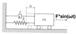
Figure: A simple 1-DOF spring damper mass system
In MATLAB, 1-DOF m-c-k system is analyzed by in time domain including the amplitude of transient part and stationary part as well as the amplitude after FFT in frequency domain.
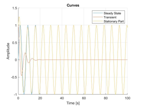
Figure: Amplitude of 1-DOF in time domain
With the aid of FFT, those extra disturbance with their amplitudes and a series of frequencies can also be clearly drawn at the bottom of horizontal axis. For narrow banded process and broad banded process, in time domain, narrow band can be clearly distinguished and all frequencies are in narrow frequency band; instead, broad band is in a mess when signals are mixed with different frequencies. It is difficult to ensure zero mean as it varies over long time. In frequency domain, narrow band have smaller interval (0-25Hz) in frequency domain and broad band has larger interval(0-100Hz) which causes some signals difficult to capture. The following figures have validated the description.
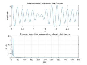
Figure: narrow banded process
Window function can help us filter signals with leakage to other period which causes an effect of addition, and therefore it can ensure that only limited signal within the original bandwidth is captured. In following figure, we can see that signal with disturbance is clearer in the higher amplitude, though there are some burrs still existed. Anyway, the signal is distributed between 0-20 Hz.
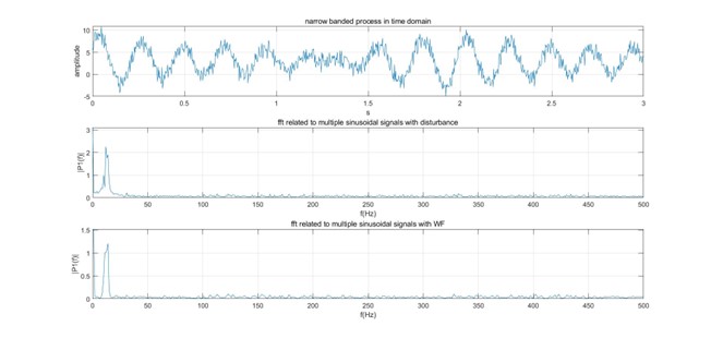
Figure: narrow banded process and its effect with Window Function
In comparison with narrow band, broad banded process has an obvious effect with window function. Signals are limited to small range of frequencies.
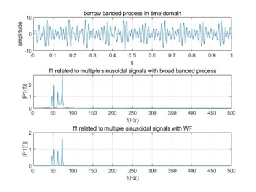
Figure: broad banded process and its effect with Window Function
Additionally, when getting the road spectrum, analysis of model was from theory to practical phase. From the state-space formula, the transfer function of random loading could be inferred. The value of the following figures, which are RAO and the response of load spectrum, can be computed. After that, we can get the figure of Response of the system for random loading shown as following figure, which is narrow band since the signal is in a smaller frequency interval. The physical meaning of the response spectrum is to reflect the degree of volatility of a specific road profile.
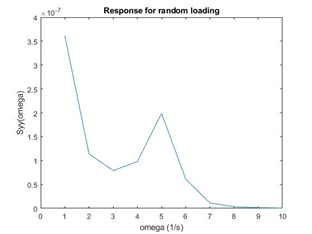
Figure: response of the system for random loading
As for the function of mean value, standard deviation and autocorrelation, I think they can help us to validate reliability of stochastic process and in the assignment, it can been seen that mean value and deviation of loading process have slight fluctuation in time averages. Instead, mean value and standard deviation of response of the suspension system have larger changes during time sequences. These results suggest that the random loading is a relatively stochastic process and the response of system is not a pure stochastic process. I think the reason can be ascribed to those assumptions we set and those conditions we simplify.
From the angle of autocorrelation, either in loading process or in response process with each other, it is shown that at some period, the value of autocorrelation fluctuates over zero and slowly changes with time going by. Its value of road loading is smaller than system response and it mentions again that the process of road loading is more stochastic than the process of system response. Additionally, we also fit the curve with estimated data, and the gaussian distribution is plotted with variable of road elevation.
Additionally, we also fit the curve with estimated data, and the gaussian distribution is plotted with variable of road elevation (in system response only partial data in stationary state expressed by normal distribution). Actually, what is the best method to express the probability distribution? From the fit of our data in assignment, the optimal method is normal to fit the curve. It is because we do not know the exact order of equation and there is more or less redundancy or exceedance of degree. However, we can increase the interpolation points to minimize the error even with poly function to fit the curve. The compared effect can be seen as following figure.
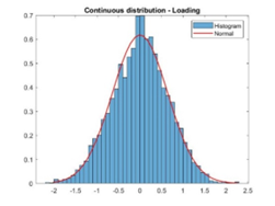
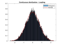
Figure: Rayleigh distribution with little interpolation points in Rainflow cycle counting
Figure: Rayleigh distribution with adequate interpolation points in Rainflow cycle counting
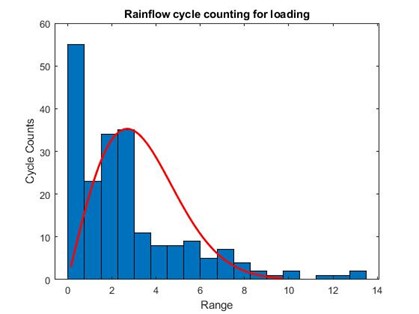
Figure: Rayleigh distribution with interpolation points in Rainflow cycle counting for loading
Rainflow analysis method is used to count fatigue cycles with stress reversals from a time history and to assess the fatigue life of a structure subject in complicated loading. Figure 9Figure 10 are plotted Rainflow cycle counting for the random load signal. This is obvious because rainflow analysis counts cycles in the certain range from the signal history and we are assuming the load spectrum of the road profile analytically as exponential function. Further, road roughness is the unique factor taken into consideration and thus our assumptions are reasonable. We can image that when we drive on the road, the main elevation is road elevation but not those sudden bumps.
The meaning of this group project is to understand the comfort and oscillation, or even vehicle’s speed which is related to vehicle’s vibration frequency. When we get familiar with their relationship, it would be better for us to design or limit the road speed for vehicles.
It should be noted that the short version of this summary is concluded from my longer learning diary, which could be checked in the following link since the figures in this document are not clear.